This function generates an array of random numbers from a named probability distribution. Note that this is not currently implemented for AIX and macOS.
Y is a 2-item vector containing the name of the probability distribution from those listed in the table below, and the shape of the result.
X is a scalar or 1 or 2 element numeric vector that specifies parameters.
For example to get an array with shape (3 5 7) of uniform random numbers for the interval from ¯17.3 to 12.7, you’d enter
¯17.3 12.7 (16808 ⌶) 'Uniform' (3 5 7)
If you wanted a vector of 100,000 uniform random numbers for that interval, you’d enter
¯17.3 12.7 (16808 ⌶) 'Uniform' 100000
The domain rules for the distributions currently implemented are as follows:
| Distribution | X[1] | X[2] | Domain Rules |
|---|---|---|---|
| 'Uniform' | a | b |
a < b ; A numeric interval. Example: 1.0 7.6 |
| 'Beta' | a | b | a > 0 AND b > 0 |
| 'Bernoulli' | probability | probability ≥ 0 AND probability ≤ 1 |
|
| 'Binomial' | trials | probability |
trials is an integer ≥ 0; probability ≥ 0 AND probability ≤ 1 |
| 'Cauchy' | location | scale |
location unrestricted; scale > 0 |
| 'Chi Squared' | degree of freedom | degree of freedom ≥ 0 | |
| 'Exponential' | rate | rate ≥ 0 | |
| 'F' | a | b |
a ≥ eps AND b ≥ eps; where eps is smallest non-zero positive float number |
| 'Gamma' | a | b |
a ≥ 0 AND b ≥eps; where eps is smallest non-zero positive float number |
| 'Inverse Gamma' | a | b | a ≥ 0 AND b ≥ 0 |
| 'Laplace' | location | scale |
location unrestricted; scale ≥ 0 |
| 'Logistic' | location | scale | location unrestricted; scale ≥ 0 |
| 'Log Normal' | location | scale | location unrestricted; scale ≥ 0 |
| 'Normal' | location | scale | location unrestricted; scale ≥ 0 |
| 'Poisson' | rate | rate ≥ 0 | |
| 'Student T' | degree of freedom |
degree of freedom ≥eps where eps is smallest non-zero positive float number |
|
| 'Weibull' | a | b | a ≥ eps AND b ≥ eps ; eps is smallest non-zero positive float number |
Each of those distributions has a corresponding Wikipedia entry with a description of its theoretical foundation and usually graphs of the probability density functions and cumulative distribution functions for interesting sets of parameter values.
Example
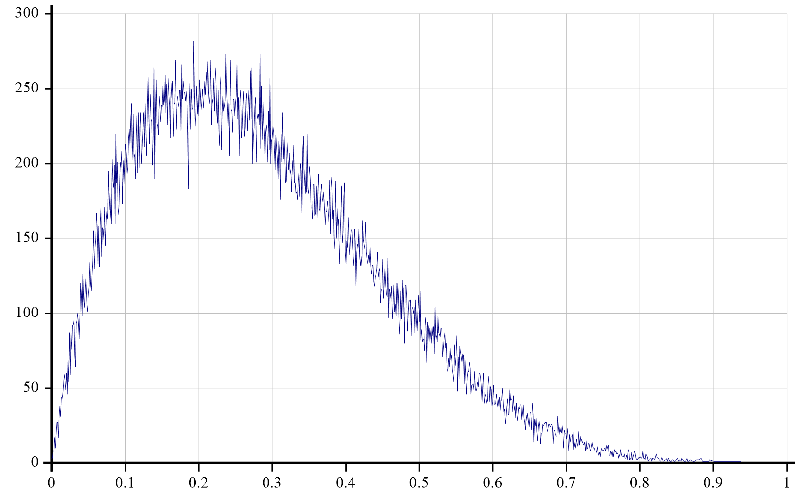
The probability density function for the Beta distribution (see https://en.wikipedia.org/wiki/Beta_distribution) with the parameter vector (2 5) has an interesting shape.
BucketCount counts random numbers that fall into a sequence of evenly distributed bucket intervals:
      BucketCounts←{
[1]        ir←⌊⍵÷÷⍺
[2]        kir←{⍺(≢⍵)}⌸ir
[3]        kir[;⎕IO]÷←⍺
[4]        kir[⍋kir[;⎕IO];]
[5]    }
So then we can create 100,000 samples and calculate values for a density graph with 1,000 evenly spaced buckets by:
      rv←2 5 (16808⌶)'Beta' 100000
      bc←1000 BucketCounts rv
Using the Chart Wizard ![]() we can plot (⊂2)⌷⍉bc against (⊂1)⌷⍉bc to get the graph:
we can plot (⊂2)⌷⍉bc against (⊂1)⌷⍉bc to get the graph:
